The Bootstrap Chain Ladder from Scratch using Polars
The bootstrap chain ladder from scratch using polars
Python
Actuarial
Published
January 25, 2025
In an earlier post, I provided a step-by-step guide on performing the bootstrap chain ladder using Pandas. This method involves repeatedly resampling residuals from the original chain ladder model to generate a series of simulated datasets, each replicating the original data’s claims development patterns (for more background, refer to the linked article).
Here we again walkthrough the bootstrap chain ladder step-by-step, this time using Polars, a high-performance DataFrame library built in Rust specifically designed for efficient data processing with large datasets. Unlike Pandas which is single-threaded, Polars leverages multi-core processors resulting in faster execution for many tasks. Although not required for our work in this setting, Polars can also handle datasets larger than available memory, spilling to disk when necessary. In Pandas, we can only process datasets having size less than or equal to available system memory.
Although Polars offers clear advantages over Pandas in many scenarios, this particular case isn’t one of them. Polars eliminates the concept of an index, which is a core feature of Pandas. But indices are especially valuable in this context for calculating age-to-age factors, identifying values along the latest diagonal, and squaring triangles. Additionally, while some insurers may store tens or hundreds of millions of claim records in their data warehouses, losses are typically aggregated by origin and development period ahead of a reserving analysis, resulting in datasets greatly reduced in size vs. transactional claim data. As a consequence, reserving actuaries typically don’t work with datasets large enough to necessitate parallel processing or out-of-core computation.
Translating the original Pandas bootstrap chain ladder code to Polars provided a good opportunity to showcase the library’s core features. However, many operations felt much less intuitive compared to their Pandas counterparts. Even so, I see this post as a valuable reference for specific Polars operations that I’ll likely use again in the future.
The steps to perform the bootstrap chain ladder:
Transform loss data into cumulative triangle representation.
Calculate the cumulative fitted triangle by applying backwards recursion, beginning with the observed cumulative losses from the latest diagonal.
Calculate the unscaled Pearson residuals, \(r_{p}\), degrees of freedom \(DF\) and scale parameter \(\phi\).
Calculate the adjusted Pearson residuals, defined as \(r_{p}^{{adj}} = \sqrt{\frac{n}{DF}} \times r_{p}\).
For each bootstrap sample (1…1000):
Generate a sample from the adjusted Pearson residuals \(r_{p}^{{adj}}\) with replacement.
Using the sampled adjusted Pearson residuals and fitted incremental triangle \(m\), construct the triangle of sampled incremental losses \(I_{i} = m + \hat{r}_{p}^{adj} \sqrt{m}\), where \(\hat{r}_{p}^{adj}\) represents a sample with replacement from the adjusted Pearson residuals and \(m\) the fitted incremental triangle.
Create a cumulative triangle using the result from ii., and project future losses using the chain ladder method.
Incorporate process variance by simulating each future projected incremental loss from a gamma distribution parameterized with mean equal to the projected loss value and variance the loss value times \(\phi\).
Cumulate the incremental losses, then compute the total needed reserve as the ultimate projected value minus the latest cumulative loss amount by origin period.
Compute desired quantiles of interest from predictive distribution of bootstrap samples.
In what follows each step is demonstrated, along with exhibits to visually assess the distribution of future losses.
%load_ext watermarkimport warningsimport matplotlib.pyplot as pltimport numpy as npimport pandas as pdimport polars as plnp.set_printoptions(suppress=True, precision=5)pd.set_option("display.precision", 5)pd.options.mode.chained_assignment =Nonepd.set_option('display.max_columns', None)pd.set_option('display.width', None)warnings.simplefilter(action="ignore", category=FutureWarning)pl.Config(tbl_rows=30)pl.Config(float_precision=4)pl.Config(tbl_cols=None)%watermark --python --conda --hostname --machine --iversions
Python implementation: CPython
Python version       : 3.12.8
IPython version      : 8.31.0

conda environment: polars

Compiler    : MSC v.1942 64 bit (AMD64)
OS          : Windows
Release     : 11
Machine     : AMD64
Processor   : Intel64 Family 6 Model 170 Stepping 4, GenuineIntel
CPU cores   : 22
Architecture: 64bit

Hostname: JTRIZPC11

matplotlib: 3.10.0
pandas    : 2.2.3
polars    : 1.20.0
numpy     : 2.2.2
Start by loading the data from GitHub:
# Load RAA dataset. dfraa = pl.read_csv("https://gist.githubusercontent.com/jtrive84/976c80786a6e97cce7483e306562f85b/raw/06a5c8b1f823fbe2b6da15f90a672517fa5b4571/RAA.csv")dfraa = dfraa.sort(by=["ORIGIN", "DEV"])print("Original incremental loss data:")# Subtract 1980 from ORIGIN.dfraa = dfraa.with_columns(pl.col("ORIGIN").sub(1980).alias("ORIGIN"))dfraa.head(10)
Original incremental loss data:
shape: (10, 3)
ORIGIN
DEV
VALUE
i64
i64
i64
1
1
5012
1
2
3257
1
3
2638
1
4
898
1
5
1734
1
6
2642
1
7
1828
1
8
599
1
9
54
1
10
172
A number of functions are defined that will be used throughout the remainder of the article. Note that the implementations differ from the Pandas version: to_cum and to_incr accept an optional as_tri argument, which when set to True transforms the table of losses into a DataFrame formatted as a runoff triangle:
to_cum: Accepts an incremental loss DataFrame and returns a cumulative loss DataFrame, optionally structured as a runoff triangle.
to_incr: Accepts a cumulative loss DataFrame and returns an incremental loss DataFrame, optionally structured as a runoff triangle.
get_a2a_factors: Accepts a cumulative triangle and returns the all-year volume weighted age-to-age factors.
get_latest: Accepts a triangle and returns the value at the latest development period by origin.
square_tri: Accepts a cumulative triangle and set of age-to-age factors and projects future losses, populating the lower-right of the original cumulative triangle.
For get_a2a_factors, get_latest and square_tri, a few simplifying assumptions have been made:
The triangles under consideration have an equal number of development and origin periods.
Development periods are sequential starting with 1.
No tail factor is included.
def to_tri(df: pl.DataFrame) -> pl.DataFrame:""" Return DataFrame structured as runoff triangle. Args: df: pd.DataFrame Loss data with columns ORIGIN, DEV and VALUE. Returns: pl.DataFrame """return df.pivot(index="ORIGIN", on="DEV", values="VALUE")def to_table(tri: pl.DataFrame) -> pl.DataFrame:""" Accepts a DataFrame structured as a triangle and returns the tabular representation having columns ORIGIN, DEV and VALUE. Args: df: pd.DataFrame Loss data structures as a runoff triangle. Returns: pl.DataFrame """ df = tri.unpivot(tri.columns[1:], index=["ORIGIN"], variable_name="DEV", value_name="VALUE") df = df.with_columns(pl.col("DEV").cast(pl.Int32).alias("DEV")) df = df.sort(["ORIGIN", "DEV"])return dfdef to_cum(df: pl.DataFrame, as_tri: bool=False) -> pl.DataFrame:""" Accepts a DataFrame of incremental losses and returns a DataFrame of cumulative losses. Optionally return DataFrame as cumulative triangle. Args: df : pl.DataFrame Incremental losses. as_tri: bool Should DataFrame be returned as a triangle. Returns: pl.DataFrame """ dfc = df.with_columns( pl.col("VALUE").cum_sum().over("ORIGIN").alias("VALUE") )if as_tri:return to_tri(dfc)else:return dfcdef to_incr(df: pl.DataFrame, as_tri: bool=False) -> pl.DataFrame:""" Accepts a DataFrame with cumulative losses and de-cumulates. Args: ctri : pl.DataFrame Cumulative losses. as_tri : bool Should DataFrame be returned as a triangle. Returns: pl.DataFrame """# Get values at first development period. first_devp_values = df.filter(pl.col("DEV")==1).select("VALUE").to_numpy().flatten()# Compute difference of cumulative losses by each origin period. df = df.with_columns(VALUE=(pl.col("VALUE").diff()).over("ORIGIN"))if as_tri:# Convert to triangle. tri = to_tri(df)# Set first development period to first_devp_values. tri = tri.with_columns(pl.Series("1", first_devp_values))return trielse:return dfdef get_a2a_factors(tri: pl.DataFrame) ->list[tuple[str, float]]:""" Calculate all-year volume weighted age-to-age factors. Args: tri: pl.DataFrame Cumulative triangle. Returns: List of (age-to-age header, age-to-age factor). """ max_origin = ctri0["ORIGIN"].max() all_devps = tri.columns[1:] dps0, dps1 = all_devps[:-1], all_devps[1:] a2a_headers = [f"{ii}-{jj}"for ii, jj inzip(dps0, dps1)] a2a = []for dp0, dp1 inzip(reversed(dps0), reversed(dps1)): v1 = tri.select(str(dp0)).to_numpy().flatten()[:(max_origin -int(dp1) +1)] v2 = tri.select(str(dp1)).to_numpy().flatten()[:(max_origin -int(dp1) +1)] a2a.append((np.nansum(v2) / np.nansum(v1)).item())returnlist(zip(a2a_headers, a2a[::-1]))def get_latest(tri: pl.DataFrame) ->list[tuple[str, float]]:""" Return the value at the latest development period by origin. Args: tri : pl.DataFrame Cumulative or incremental triangle. Returns: list of (origin, latest) tuples. """if"ORIGIN"in tri.columns: tri = tri.drop("ORIGIN") nbr_devps = tri.width latest = [tri[ii, nbr_devps - ii -1] for ii inrange(nbr_devps)]returnlist(zip(tri.columns, latest))def square_tri(tri: pl.DataFrame, a2a: list[tuple[str, float]]) -> pl.DataFrame:""" Project future losses for `tri` using `a2a`. Args: tri : pl.DataFrame Cumulative triangle. a2a: list Age-to-age factors. Returns ------- pl.DataFrame Original triangle with projected future losses. """if"ORIGIN"in tri.columns: sqrd = tri.drop("ORIGIN")else: sqrd = tri _, a2a_values =zip(*a2a) nbr_devps = sqrd.widthfor r_idx inrange(nbr_devps):for c_idx inrange(nbr_devps - r_idx, nbr_devps): sqrd[r_idx, str(c_idx +1)] = sqrd[r_idx, str(c_idx)] * a2a_values[c_idx -1] sqrd = sqrd.with_row_index("ORIGIN", offset=1)return sqrd
Create an incremental loss triangle, passing dfraa into to_tri:
tri0 = to_tri(dfraa)print("Original incremental loss triangle:")tri0
Original incremental loss triangle:
shape: (10, 11)
ORIGIN
1
2
3
4
5
6
7
8
9
10
i64
i64
i64
i64
i64
i64
i64
i64
i64
i64
i64
1
5012
3257
2638
898
1734
2642
1828
599
54
172
2
106
4179
1111
5270
3116
1817
-103
673
535
null
3
3410
5582
4881
2268
2594
3479
649
603
null
null
4
5655
5900
4211
5500
2159
2658
984
null
null
null
5
1092
8473
6271
6333
3786
225
null
null
null
null
6
1513
4932
5257
1233
2917
null
null
null
null
null
7
557
3463
6926
1368
null
null
null
null
null
null
8
1351
5596
6165
null
null
null
null
null
null
null
9
3133
2262
null
null
null
null
null
null
null
null
10
2063
null
null
null
null
null
null
null
null
null
Next we create a cumulative loss triangle using to_cum with as_tri = True:
ctri0 = to_cum(dfraa, as_tri=True)print("Original cumulative loss triangle:")ctri0
Original cumulative loss triangle:
shape: (10, 11)
ORIGIN
1
2
3
4
5
6
7
8
9
10
i64
i64
i64
i64
i64
i64
i64
i64
i64
i64
i64
1
5012
8269
10907
11805
13539
16181
18009
18608
18662
18834
2
106
4285
5396
10666
13782
15599
15496
16169
16704
null
3
3410
8992
13873
16141
18735
22214
22863
23466
null
null
4
5655
11555
15766
21266
23425
26083
27067
null
null
null
5
1092
9565
15836
22169
25955
26180
null
null
null
null
6
1513
6445
11702
12935
15852
null
null
null
null
null
7
557
4020
10946
12314
null
null
null
null
null
null
8
1351
6947
13112
null
null
null
null
null
null
null
9
3133
5395
null
null
null
null
null
null
null
null
10
2063
null
null
null
null
null
null
null
null
null
Calculate the all-year volume weighted age-to-age factors
Calculate the cumulative fitted triangle by applying backwards recursion, beginning with the observed cumulative losses from the latest diagonal.
nbr_devps = ctri0.width -1a2a_headers, a2a_values =zip(*a2a)# Create empty triangle with same shape as ctri0. ctri = pl.DataFrame( {f"{i}": [np.nan] * nbr_devps for i inrange(1, 11)}).with_row_index("ORIGIN", offset=1)for r_idx inrange(ctri["ORIGIN"].shape[0]):# Determine latest development period. latest_devp = nbr_devps - r_idx# Set latest diagonal of tri to same value as in tri0. ctri[r_idx, str(latest_devp)] = ctri0[r_idx, str(latest_devp)] # Use backward recursion to un-develop triangle using a2a_values. for devp inrange(latest_devp -1, 0, -1): ctri[r_idx, str(devp)] = (ctri[r_idx, str(devp +1)] / a2a_values[devp -1])print("Fitted cumulative triangle:")ctri
Fitted cumulative triangle:
shape: (10, 11)
ORIGIN
1
2
3
4
5
6
7
8
9
10
u32
f64
f64
f64
f64
f64
f64
f64
f64
f64
f64
1
2111.3796
6332.7847
10281.4201
13066.5346
15309.7271
17045.6188
17760.4206
18351.1953
18662.0000
18834.0000
2
1889.8556
5668.3547
9202.7029
11695.6057
13703.4445
15257.2080
15897.0135
16425.8047
16704.0000
NaN
3
2699.8587
8097.8445
13147.0348
16708.4103
19576.8205
21796.5360
22710.5659
23466.0000
NaN
NaN
4
3217.7567
9651.2063
15668.9531
19913.4862
23332.1267
25977.6372
27067.0000
NaN
NaN
NaN
5
3242.8226
9726.3881
15791.0124
20068.6100
23513.8813
26180.0000
NaN
NaN
NaN
NaN
6
2186.1650
6557.0929
10645.5896
13529.3532
15852.0000
NaN
NaN
NaN
NaN
NaN
7
1989.7800
5968.0637
9689.2872
12314.0000
NaN
NaN
NaN
NaN
NaN
NaN
8
2692.6640
8076.2650
13112.0000
NaN
NaN
NaN
NaN
NaN
NaN
NaN
9
1798.7179
5395.0000
NaN
NaN
NaN
NaN
NaN
NaN
NaN
NaN
10
2063.0000
NaN
NaN
NaN
NaN
NaN
NaN
NaN
NaN
NaN
Calculate the unscaled Pearson residuals, \(r_{p}\), degrees of freedom \(DF\) and scale parameter \(\phi\).
The unscaled Pearson residuals are defined as
\[
r_{p} = \frac{I - m}{\sqrt{m}},
\]
where \(I\) represents actual incremental losses and \(m\) fitted incremental losses.
Polars doesn’t have an equivalent to Pandas df.diff(axis=1), so the implementation of to_incr is a little more involved than what we saw last post. First, the actual triangle on incremental losses:
The unscaled Pearson residuals are then calculated element-wise:
numer = tri0.select(tri0.columns[1:]) - tri.select(tri.columns[1:]) denom = tri.select(pl.col(tri0.columns[1:]).abs().sqrt())r_us = numer / denomprint("Unscaled Pearson residuals:")r_us
Unscaled Pearson residuals:
shape: (10, 10)
1
2
3
4
5
6
7
8
9
10
f64
f64
f64
f64
f64
f64
f64
f64
f64
f64
63.1259
-14.8433
-20.8573
-35.7583
-10.7510
21.7480
41.6370
0.3384
-14.5666
0.0000
-41.0341
6.5154
-40.7625
55.6209
24.7308
6.6781
-29.3664
6.2712
15.3967
null
13.6670
2.5046
-2.3670
-21.6728
-5.1237
26.7285
-8.7663
-5.5461
null
null
42.9657
-6.6508
-23.2906
19.2704
-21.5437
0.2428
-3.1923
null
null
null
-37.7697
24.7072
2.6501
31.4266
5.8049
-47.2769
null
null
null
null
-14.3973
8.4866
18.2746
-30.7401
12.3326
null
null
null
null
null
-32.1201
-8.1696
52.5357
-24.5299
null
null
null
null
null
null
-25.8555
2.8948
15.9135
null
null
null
null
null
null
null
31.4605
-22.2495
null
null
null
null
null
null
null
null
0.0000
null
null
null
null
null
null
null
null
null
\(DF = n - p\), where \(n\) is the number of populated cells in the original triangle and \(p\) the number of parameters in the chain ladder model (10 for origin period and 9 for development period):
n = tri0.count().sum().to_numpy().flatten()[1:].sum().item()p = tri0.height + tri0.width -2DF = n - pprint(f"Degrees of freedom: {DF}.")
Degrees of freedom: 36.
The scale parameter \(\phi\) is the sum of the squared unscaled Pearson residuals over the degrees of freedom:
(From this point each subsequent step is repeated up to the desired number of bootstrap samples.)
Generate a sample from the adjusted Pearson residuals with replacement:
# Set random seed for reproducibility.rng = np.random.default_rng(seed=516)# Represent adjusted residuals as Numpy array with nans and 0s removed.r = r_adj[:-1, :-1].to_numpy().flatten()r = r[np.logical_and(~np.isnan(r), r !=0)] # Sample tri0.shape[0] * tri0.shape[1] values at each iteration, but only# keep values in upper left portion of triangle. Use mask to determine # which values to retain.mask =~np.isnan(tri[:,1:])# Sample with replacement from adjusted residuals. s_r = rng.choice(r, size=mask.shape, replace=True)# # Replace 0s with nans.s_r = mask * s_rs_r[s_r==0] = np.nans_r = pl.from_numpy(s_r, schema=[str(i) for i inrange(1, 11)])print("Sample with replacement from adjusted Pearson residuals:")s_r
Sample with replacement from adjusted Pearson residuals:
shape: (10, 10)
1
2
3
4
5
6
7
8
9
10
f64
f64
f64
f64
f64
f64
f64
f64
f64
f64
-50.3838
-13.2886
7.1751
30.5389
26.8812
-18.3468
-58.4358
33.0374
10.4897
7.1751
-10.0978
8.2544
-26.7883
0.4183
78.0257
-58.4358
38.8443
-30.3197
19.6696
NaN
-27.5012
38.8443
-58.4358
-6.3330
7.1751
-27.5012
0.4183
-50.7196
NaN
NaN
-44.1984
8.0533
-37.9958
-27.5012
38.8443
-25.7803
-30.3197
NaN
NaN
NaN
19.0308
-3.9458
-26.7883
-2.9256
38.8863
7.7514
NaN
NaN
NaN
NaN
30.5681
-27.5012
26.8812
8.2544
38.8443
NaN
NaN
NaN
NaN
NaN
-39.7015
-17.7955
-18.3468
-10.8354
NaN
NaN
NaN
NaN
NaN
NaN
22.5880
-18.0048
3.0957
NaN
NaN
NaN
NaN
NaN
NaN
NaN
-25.7803
-26.7883
NaN
NaN
NaN
NaN
NaN
NaN
NaN
NaN
0.4183
NaN
NaN
NaN
NaN
NaN
NaN
NaN
NaN
NaN
Using the sampled adjusted Pearson residuals and fitted incremental triangle \(m\), construct the triangle of sampled incremental losses \({I_{i}}\):
\[
I_{i} = m + \hat{r}_{p}^{adj} \sqrt{m},
\]
where \(\hat{r}_{p}^{adj}\) represents a sample with replacement from the adjusted Pearson residuals and \(m\) the fitted incremental triangle:
tri_ii = tri[:,1:] + s_r * tri.select(pl.col(tri.columns[1:]).sqrt())tri_ii = tri_ii.with_row_index("ORIGIN", offset=1)print("Triangle of sampled incremental loss tri_ii:")tri_ii
Triangle of sampled incremental loss tri_ii:
shape: (10, 11)
ORIGIN
1
2
3
4
5
6
7
8
9
10
u32
f64
f64
f64
f64
f64
f64
f64
f64
f64
f64
1
-203.7452
3358.0144
4399.5047
4396.7778
3516.3502
971.4887
-847.5257
1393.7759
495.7340
266.1004
2
1450.8774
4285.8909
1941.7709
2513.7873
5504.0870
-749.6490
1622.3472
-168.4248
606.2675
NaN
3
1270.8943
8251.9128
896.8769
3183.4392
3252.6902
924.0302
926.6758
-638.6012
NaN
NaN
4
710.5888
7079.3951
3070.2582
2452.8309
5689.8317
1319.5115
88.6453
NaN
NaN
NaN
5
4326.5491
6165.8502
3978.4635
4086.2513
5727.7564
3066.3579
NaN
NaN
NaN
NaN
6
3615.4212
2552.7444
5807.3180
3327.0288
4194.7016
NaN
NaN
NaN
NaN
NaN
7
218.8165
2855.8569
2602.0332
2069.5944
NaN
NaN
NaN
NaN
NaN
NaN
8
3864.7765
4062.5315
5255.4183
NaN
NaN
NaN
NaN
NaN
NaN
NaN
9
705.3407
1989.8118
NaN
NaN
NaN
NaN
NaN
NaN
NaN
NaN
10
2081.9985
NaN
NaN
NaN
NaN
NaN
NaN
NaN
NaN
NaN
Create a cumulative triangle, and project future losses using the chain ladder method:
# Create cumulative triangle from sampled incremental losses.ctri_ii = to_cum(to_table(tri_ii), as_tri=True)# Get age-to-age factors for sampled cumulative triangle.a2a_ii = get_a2a_factors(ctri_ii)# Square ctri_ii, populating the lower-right side using a2a_ii.ctri_ii_sqrd = square_tri(ctri_ii, a2a_ii)print("Completed sampled triangle ctri_ii_sqrd:")ctri_ii_sqrd
Completed sampled triangle ctri_ii_sqrd:
shape: (10, 11)
ORIGIN
1
2
3
4
5
6
7
8
9
10
u32
f64
f64
f64
f64
f64
f64
f64
f64
f64
f64
1
-203.7452
3154.2692
7553.7739
11950.5517
15466.9019
16438.3906
15590.8649
16984.6408
17480.3748
17746.4752
2
1450.8774
5736.7683
7678.5392
10192.3265
15696.4135
14946.7645
16569.1116
16400.6868
17006.9544
17265.8480
3
1270.8943
9522.8071
10419.6840
13603.1232
16855.8134
17779.8436
18706.5194
18067.9182
18664.3141
18948.4374
4
710.5888
7789.9839
10860.2421
13313.0730
19002.9047
20322.4162
20411.0615
20646.5050
21328.0164
21652.6887
5
4326.5491
10492.3993
14470.8628
18557.1141
24284.8704
27351.2284
28055.8538
28379.4807
29316.2465
29762.5220
6
3615.4212
6168.1656
11975.4836
15302.5124
19497.2140
20678.4336
21211.1538
21455.8265
22164.0523
22501.4514
7
218.8165
3074.6735
5676.7067
7746.3011
10351.3688
10978.4964
11261.3256
11391.2261
11767.2341
11946.3644
8
3864.7765
7927.3080
13182.7263
17413.9552
23270.2385
24680.0431
25315.8531
25607.8739
26453.1529
26855.8442
9
705.3407
2695.1525
4093.6863
5407.6272
7226.2030
7663.9954
7861.4361
7952.1185
8214.6065
8339.6559
10
2081.9985
7378.7321
11207.6084
14804.8883
19783.7469
20982.3259
21522.8749
21771.1433
22489.7774
22832.1349
So far we’ve accounted for parameter variance, but not process variance. In order to obtain the full prediction error, we need to incorporate process variance into our estimates. This is accomplished by simulating incremental projected losses from a gamma distribution. For each cell in the lower right of the completed triangle, we randomly sample from a gamma distribution with mean equal to the projected incremental loss in that cell, and variance equal to the value in that cell times \(\phi\). For example, consider the following squared incremental triangle:
Values to the right of the main diagonal represent projected future losses. For the loss at origin = 2000 and development period = 2, the projected incremental loss is 17. We would therefore sample from a gamma distribution parameterized as follows:
from numpy.random import gamma# Computed above. phi =.798# Value at intersection of origin=2000 and development period = 2.mu =17# Determine shape and scale from mean and variance.shape = mu**2/ (phi * mu)scale = (phi * mu) / mu# Generate sample from gamma distribution.rng.gamma(shape=shape, scale=scale, size=1)# array([19.29149])
We take advantage of the fact that for the gamma distribution, the shape parameter \(\alpha = E[X]^{2} / \mathrm{Var}[X]\) and scale \(\theta = \mathrm{Var}[X] / E[X]\). In essence, we are simulating future incremental losses from a series a gamma distributions, each with parameterization based on the chain ladder-derived future incremental losses. To handle cases in which a projected incremental loss might be negative, we take the absolute value of the projected loss when determining \(\alpha_{ij}\) and \(\theta_{ij}\) for origin period \(i\), development period \(j\), where \(2 \leq i \leq n\) and \(j \geq n - i + 2\).
"""Incorporation of process variance. """from numpy.random import gamma# Get sampled squared incremental triangle.tri_ii_sqrd = to_incr(to_table(ctri_ii_sqrd), as_tri=True).drop("ORIGIN")for r_idx inrange(nbr_devps):for c_idx inrange(nbr_devps - r_idx, nbr_devps):# Get mean and variance using incremental loss value. m = np.abs(tri_ii_sqrd[r_idx, str(c_idx)]) v = m * phi# Determine shape and scale parameters. shape = m**2/ v scale = v / m# Update value at [r_idx, c_idx] with sample from gamma distribution. tri_ii_sqrd[r_idx, str(c_idx)] = rng.gamma(shape=shape, scale=scale, size=1).item()print("Sampled incremental triangle w/ process variance:")tri_ii_sqrd
Sampled incremental triangle w/ process variance:
shape: (10, 10)
1
2
3
4
5
6
7
8
9
10
f64
f64
f64
f64
f64
f64
f64
f64
f64
f64
-203.7452
3358.0144
4399.5047
4396.7778
3516.3502
971.4887
-847.5257
1393.7759
495.7340
266.1004
1450.8774
4285.8909
1941.7709
2513.7873
5504.0870
-749.6490
1622.3472
-168.4248
5.6818
258.8936
1270.8943
8251.9128
896.8769
3183.4392
3252.6902
924.0302
926.6758
261.2162
45.4568
284.1233
710.5888
7079.3951
3070.2582
2452.8309
5689.8317
1319.5115
0.0000
1187.7049
138.5052
324.6723
4326.5491
6165.8502
3978.4635
4086.2513
5727.7564
2287.3879
375.7417
20.5246
624.2870
446.2756
3615.4212
2552.7444
5807.3180
3327.0288
3960.9182
218.8131
10.1640
14.2730
306.6162
337.3991
218.8165
2855.8569
2602.0332
1195.7353
962.9821
160.2781
418.3009
0.0000
14.9545
179.1303
3864.7765
4062.5315
8917.8595
1226.2463
3936.2469
2824.7474
827.3206
4.3581
84.7208
402.6913
705.3407
1146.8776
1215.0414
619.7826
3797.3911
796.3057
8.3274
2.0791
0.2504
125.0494
2713.2565
3260.8427
1892.6994
2777.3152
1124.3156
720.6907
10.0764
7.8274
299.7176
342.3576
From this point, we proceed exactly as if performing a standard chain ladder analysis: Cumulate incremental losses, then compute the total needed reserve as the ultimate projected value minus the latest cumulative loss amount by origin period. In the next cell we convert latest_values to a numpy array to simplify differencing with ultimates, but this can also be computed element-wise in a list comprehension:
The preceding steps are repeated for the desired number of bootstrap samples, resulting in the predictive distribution of total needed reserve by origin period and in aggregate.
Bringing it All Together
The steps outlined above are combined in the next cell to run 1000 bootstrap iterations, generating the predictive distribution of reserves. We also present code to visualize the predictive distribution by origin period and in aggregate.
import matplotlib.pyplot as pltimport numpy as npfrom numpy.random import gammaimport polars as plnp.set_printoptions(suppress=True, precision=5)pl.Config(tbl_rows=30)pl.Config(float_precision=4)pl.Config(tbl_cols=None)# Set random seed for reproducibility.rng = np.random.default_rng(seed=516)# Number of bootstrap samples.nbr_samples =1000# Load tabular incremental losses. Convert to incremental triangle. dfraa = pl.read_csv("https://gist.githubusercontent.com/jtrive84/976c80786a6e97cce7483e306562f85b/raw/06a5c8b1f823fbe2b6da15f90a672517fa5b4571/RAA.csv")dfraa = dfraa.sort(by=["ORIGIN", "DEV"])dfraa = dfraa.with_columns(pl.col("ORIGIN").sub(1980).alias("ORIGIN"))tri0 = to_tri(dfraa)nbr_devps = tri0.width -1mask =~np.isnan(tri0[:,1:])# Create cumulative triangle from original losses.ctri0 = to_cum(dfraa, as_tri=True)# All-year volume-weighted age-to-age factors.a2a = get_a2a_factors(ctri0)# Cumulative fitted triangle via backwards recursion.a2a_headers, a2a_values =zip(*a2a)# Create empty triangle with same shape as ctri0. ctri = pl.DataFrame( {f"{i}": [np.nan] * nbr_devps for i inrange(1, 11)}).with_row_index("ORIGIN", offset=1)for r_idx inrange(ctri["ORIGIN"].shape[0]):# Determine latest development period. latest_devp = nbr_devps - r_idx# Set latest diagonal of tri to same value as in tri0. ctri[r_idx, str(latest_devp)] = ctri0[r_idx, str(latest_devp)] # Use backward recursion to un-develop triangle using a2a_values. for devp inrange(latest_devp -1, 0, -1): ctri[r_idx, str(devp)] = (ctri[r_idx, str(devp +1)] / a2a_values[devp -1])# Incremental fitted triangle.tri = to_incr(to_table(ctri), as_tri=True)# Unscaled Pearson residuals.numer = tri0.select(tri0.columns[1:]) - tri.select(tri.columns[1:]) denom = tri.select(pl.col(tri0.columns[1:]).abs().sqrt())r_us = numer / denom# Degrees of freedom.n = tri0.count().sum().to_numpy().flatten()[1:].sum().item()p = tri0.height + tri0.width -2DF = n - p# Scale parameter.phi = r_us.with_columns(pl.all().pow(2)).sum().to_numpy().flatten().sum().item() / DF# Adjusted Pearson residuals.r_adj = np.sqrt(n / DF).item() * r_us # Create sampling distribution from adjusted Pearson residuals. Remove# nans and 0s. r = r_adj[:-1, :-1].to_numpy().flatten()r = r[np.logical_and(~np.isnan(r), r !=0)] # Sample tri0.width * tri0.height values at each iteration, but only# keep values in upper left portion of triangle. Use mask to determine # which values to retain.sqrd_ctris = []for ii inrange(nbr_samples):# Sample with replacement from adjusted residuals. s_r = rng.choice(r, size=mask.shape, replace=True) s_r = mask * s_r s_r[s_r==0] = np.nan s_r = pl.from_numpy(s_r, schema=[str(i) for i inrange(1, 11)])# Sampled incremental triangle. tri_ii = tri[:,1:] + s_r * tri.select(pl.col(tri.columns[1:]).sqrt()) tri_ii = tri_ii.with_row_index("ORIGIN", offset=1)# Sampled cumulative triangle. ctri_ii = to_cum(to_table(tri_ii), as_tri=True)# Age-to-age factors for sampled cumulative triangle. a2a_ii = get_a2a_factors(ctri_ii)# Sampled squared cumulative triangle. ctri_ii_sqrd = square_tri(ctri_ii, a2a_ii)# Sampled squared incremental triangle. tri_ii_sqrd = to_incr(to_table(ctri_ii_sqrd), as_tri=True)# Incorporate process variance.for r_idx inrange(nbr_devps):for c_idx inrange(nbr_devps - r_idx, nbr_devps):# Get mean and variance using incremental loss value. m = np.abs(tri_ii_sqrd[r_idx, str(c_idx)]) v = m * phi# Determine shape and scale parameters. shape = m**2/ v scale = v / m# Update value at [r_idx, c_idx] with sample from gamma distribution. tri_ii_sqrd[r_idx, str(c_idx)] = rng.gamma(shape=shape, scale=scale, size=1).item() ctri_ii_sqrd2 = to_cum(to_table(tri_ii_sqrd), as_tri=True)# Keep Sampled squared triangle. sqrd_ctris.append(ctri_ii_sqrd2)
Obtain the predictive distribution of reserves and ultimates from sqrd_ctris. Each triangle in sqrd_ctris is converted to a Pandas DataFrame to keep the visualization code consistent with the prior post:
Using dfults and dfibnr, we create a summary of mean ultimate, mean IBNR, standard error of IBNR as well as 75th and 95th percentiles of the predictive distribution of reserves:
from functools importreduce# Latest cumulative loss amount by origin.latest_origin, latest_values =zip(*get_latest(ctri0))latest = ( pd.Series(data=latest_values, index=[int(ii) for ii in latest_origin]) .to_frame() .reset_index(drop=False) .rename({"index": "origin", 0: "latest"}, axis=1))# Mean ultimate by origin.ult_mean = ( dfults.groupby("origin")["ult"].mean() .to_frame() .reset_index(drop=False) .rename({"ult": "ult_mean"}, axis=1))ibnr_mean = ( dfibnr.groupby("origin")["ibnr"].mean() .to_frame() .reset_index(drop=False) .rename({"ibnr": "ibnr_mean"}, axis=1))# Standard error of reserve distribution by origin. ibnr_se = ( dfibnr.groupby("origin")["ibnr"].std(ddof=1) .to_frame() .reset_index(drop=False) .rename({"ibnr": "ibnr_se"}, axis=1))# 75th percentile of reserve distribution by origin. ibnr_75 = ( dfibnr.groupby("origin")["ibnr"].quantile(.75) .to_frame() .reset_index(drop=False) .rename({"ibnr": "ibnr_75th"}, axis=1))# 95th percentile of reserve distribution by origin. ibnr_95 = ( dfibnr.groupby("origin")["ibnr"].quantile(.95) .to_frame() .reset_index(drop=False) .rename({"ibnr": "ibnr_95th"}, axis=1))# Combine into a single DataFrame.bcl_summary =reduce(lambda df1, df2: df1.merge(df2, on="origin", how="left"), (latest, ult_mean, ibnr_mean, ibnr_se, ibnr_75, ibnr_95))# Set ult_mean for earliest origin period to latest.bcl_summary.at[0, "ult_mean"] = bcl_summary.at[0, "latest"]print("Boostrap chain ladder summary by origin:")bcl_summary.round(0)
Boostrap chain ladder summary by origin:
origin
latest
ult_mean
ibnr_mean
ibnr_se
ibnr_75th
ibnr_95th
0
1
18834
18834.0
0.0
0.0
0.0
0.0
1
2
16704
17002.0
165.0
430.0
385.0
940.0
2
3
23466
24436.0
753.0
1056.0
1228.0
2719.0
3
4
27067
29034.0
1916.0
1714.0
2824.0
5079.0
4
5
26180
29014.0
2915.0
2085.0
4023.0
6865.0
5
6
15852
19656.0
3896.0
2452.0
5218.0
8692.0
6
7
12314
18031.0
5681.0
3066.0
7513.0
11501.0
7
8
13112
24818.0
11551.0
5142.0
14783.0
21143.0
8
9
5395
16291.0
10951.0
6283.0
14557.0
22634.0
9
10
2063
20003.0
17958.0
13786.0
25409.0
43653.0
While results by origin can be useful, typically actuaries are more interested in the aggregate view. To get aggregate results, we first group by simulation number, then proceed as in the prior cell:
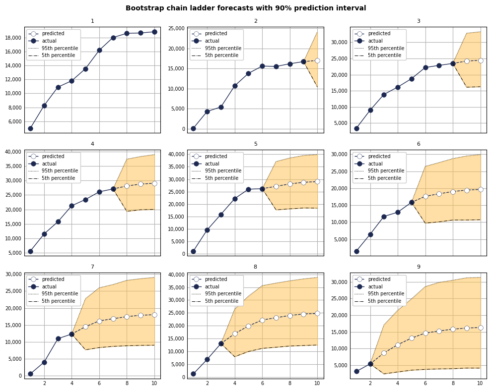
We can visualize actuals and predictions together by origin out to ultimate with 90% prediction intervals for each forecast period. Starting with sqrd_tris, we transform the data to make it easier for plotting:
dflist = []for tri in sqrd_ctris: dftri = ( tri.to_pandas().set_index("ORIGIN") .reset_index(drop=False) .rename_axis(None, axis=1) .rename({"ORIGIN": "origin"}, axis=1) .melt(id_vars="origin", var_name="dev", value_name="bcl_value") ) dflist.append(dftri)df = pd.concat(dflist)df["dev"] = df["dev"].astype(int)df = df.sort_values(["origin", "dev"]).reset_index(drop=True)# Compute mean, 5th and 95th percentile of prediction interval for each forecast period.df = ( df .groupby(["origin", "dev"], as_index=False)["bcl_value"] .agg({"bcl_mean": lambda v: v.mean(), "bcl_95th": lambda v: v.quantile(.95),"bcl_5th": lambda v: v.quantile(.05) }))# Attach actual values from original cumulative triangle.dfctri0 = ( ctri0.to_pandas().set_index("ORIGIN") .reset_index(drop=False) .rename_axis(None, axis=1) .rename({"ORIGIN": "origin"}, axis=1) .melt(id_vars="origin", var_name="dev", value_name="actual_value"))dfctri0["dev"] = dfctri0["dev"].astype(int)df = df.merge(dfctri0, on=["origin", "dev"], how="left")# If actual_value is nan, then dev is a prediction for that origin. Otherwise# it is an actual value. df["actual_devp_ind"] = df["actual_value"].map(lambda v: 1ifnot np.isnan(v) else0)df["value"] = df.apply(lambda r: r.bcl_mean if r.actual_devp_ind==0else r.actual_value, axis=1)df.tail(10)
origin
dev
bcl_mean
bcl_95th
bcl_5th
actual_value
actual_devp_ind
value
90
10
1
2044.92690
5819.41104
2.74973
2063.0
1
2063.00000
91
10
2
6523.89949
16103.08545
101.75998
NaN
0
6523.89949
92
10
3
10661.43665
25982.44515
319.20599
NaN
0
10661.43665
93
10
4
13682.08149
32977.99907
611.55764
NaN
0
13682.08149
94
10
5
16092.90839
38453.69231
799.41542
NaN
0
16092.90839
95
10
6
17973.94826
42833.83253
934.59346
NaN
0
17973.94826
96
10
7
18718.07392
45366.39099
1007.06181
NaN
0
18718.07392
97
10
8
19360.64161
46870.52200
1052.26676
NaN
0
19360.64161
98
10
9
19813.97172
47265.73702
1067.22772
NaN
0
19813.97172
99
10
10
20003.07058
47960.10396
1225.34543
NaN
0
20003.07058
Actuals with forecasts by origin year with 90% prediction intervals:
As expected, the prediction intervals grow wider for origin periods with fewer development periods of actual data to account for the greater uncertainty in ultimate projections.
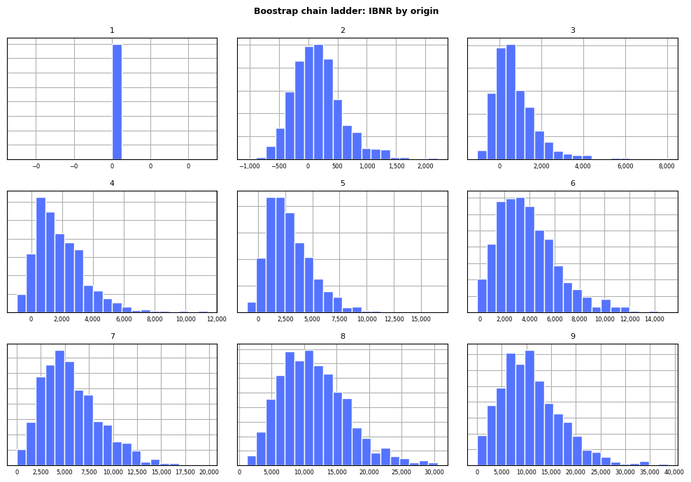
Second, an exhibit with a separate histogram per facet can be used to visualize the distribution of IBNR generated by the bootstrap chain ladder:
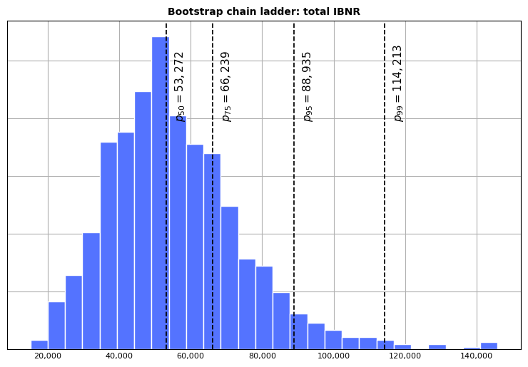
Finally, we can create a similar exhibit for the aggregate distribution of IBNR, with vertical lines added at the 50th, 75th, 95th and 99th percentile of total needed reserve: